[Note: The full report filed for the grant-funded portion of this work appears on this site at: https://brianaltonenmph.com/3-gis-environmental-health/report-for-grant-funded-research-2002/]
The Application of Nearest Neighbor/Spider Analysis to Environmental Disease Profiling
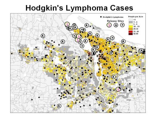
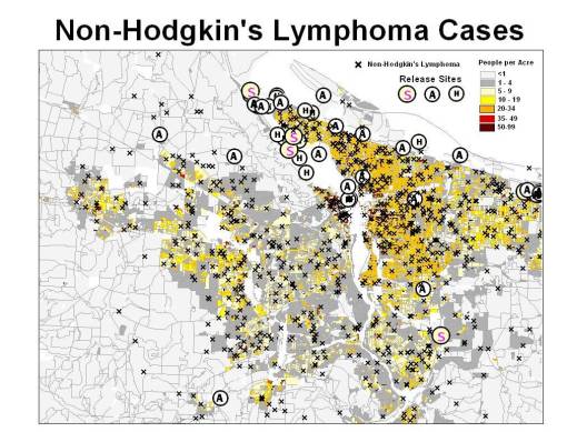
The Problem: we have two types of cancer possible that we think may be related to environmental exposure but are not certain about how to illustrate our concern using maps or how to define a way to spatially analyze these relationships.
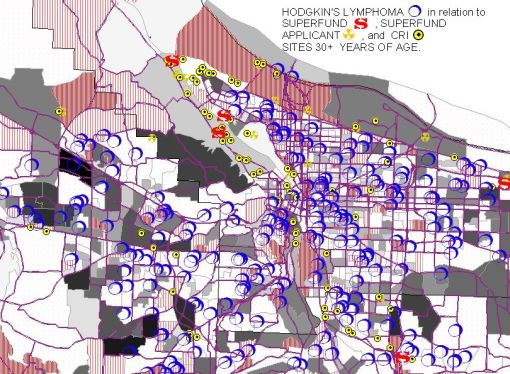
The Research Question: Do either of the above two cases demonstrate a spatial relationship with the local chemical release sites?
The traditional way to analyze these sites is to perform an incidence/prevalence-related anlysis of the cases in relation to population size for each census block area, based on specific age group sizes normalized to match state standards. This method may in fact still be one of the better ways to perform atraditional analysis of such a research question, however, an alternative method for engaging in this research is to first define the incidence rates and a census bloock level, then perform and age-adjusted analysis fo the population within each census block, and finally link this value to the block group centroid. This centroid value is then spatially analyzed in relationship to chemical release site corrdinates, and using a spider-based nearest neighbor analysis program, determine if one site or complex site area demonstrate a strong nearest neighbor relation relative to all other areas put through the same method fo areal analysis. (Note: Complex site areas are places consisting of multiple exposures, the centroid of which is defined as a point; used for closely cluster chemical release sites)
Based upon one’s first impressions after reading this method, traditional epidemiological researchers are going to criticise this method due to its lack of spatial consistency and accuracy. One could argue that by reasigning disease frequency values to a centroid offsets the actual centroids of the cases used to define the centroid value; perhaps it is better to place this number of the centroid for each cluster of cases in each block (or block group) area. The problem with this reasoning is that you introduce artificial case clustering features to a measurement that is defined by the area beneath it and the people residing within that research area. For this reason, only the areal/population centroid can and should be used to determine where you place this adjusted frequency data.
The next argument against this method is that it is not really tested, tried and proven. In fact, this method is tested and tried, and in a sense proven, for it is comparable to the methods used to cacluated frequencies based on census block data and age-adjustments performed by relating individual cases to individual population groups within a specific area. After such an analysis is performed, we then review the information spatially and determine wherre there are important outcomes. This method goes through the exact same steps, but begins with the GIS-spatial method and ends by relating the outcomes back to the population data.
Carrying this method of analysis one step further, it is better the adjust the census block numbers in such a way that true locations of residency are used, not theoretical areal-defined groups of residences all situated within one block area. In other words, block area adjustments should be made using raster/landsat/photometric data to define where exactly the residences of each area are in fact placed. In one such study I evaluated, this is possible using Landsat 7 and later imagery due to the differecnes between each image. The most important feature to correct for with residency location tools in remote sensing is the artificial or misread roof locations produced by specific land surface, such as roadways and water bodies (even very small water surfaces). Normalized difference equations were used to differentiate these features in a first attempt made to perform such a correction, suggesting with more time such a correction can actually be developed for identifying places of residence with the purpose of performing actual people-area mapping routines. (With the current technology, this is perhaps easier now.)
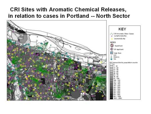
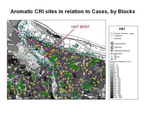
Using the census blocks for this next analysis, we find that by drawing “spiders” using an Avenue Extension tool (a series of lines all drawn towards one point from many points possibly linked to that single point), and then assigning a value to each portion of the “spider” which defines the length of the line. These values can then be compared between different multiple cases-single release site relationships, and those relationships with the closest spatial relationships compared to comparable sites in other locations can then be further analyzed.
This method is used mostly to assign priorities to certain chemical release sites. Chemical release sites with large numbers of fairly close cases are given the highest priority in exposure risk analysis. These sites may be assigned a risk value based on average spider lengths and numbers of these links established.
To perform the latter process, a simple algorithm can be used in which the 2 values (length x number) are simply multiplied. To differentiate between chemically-defined release sites and cases, a third and/or fourth multiplier may be added in which you assign higher values to increasing toxic/carcinogenic substances, and/or to their relative amounts released. These final values would be based on the numbers of substances tested for multiplied by [k x Log(amount)] for how much was actually found at the sites or centroid for combined sites.
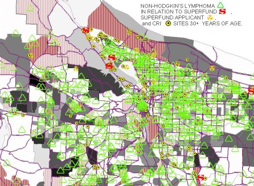
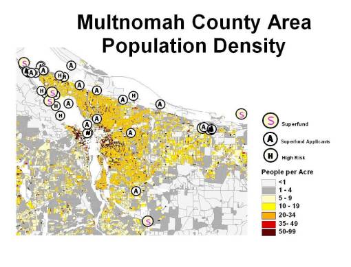
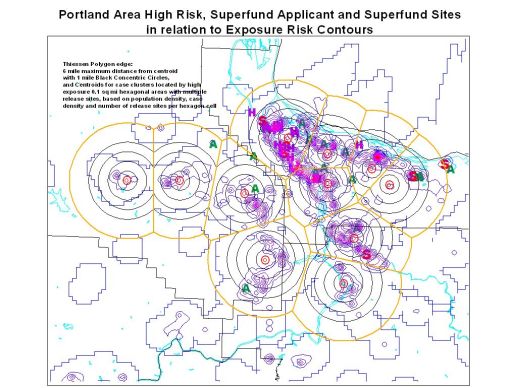
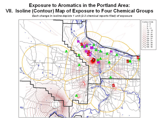
This research area has two types of spatial relationships that were of importance. The first is the relationship between the predefined high release, superfund and superfund applicants sites. The second relationship (how this was picked up appears later in the review of hexagonal grid analysis technique) adds to these basic highly toxic sites information on the remaining CRI sites and TRI sites. In the first mapped product, there are several possible sites with significant numbers of cases linked to them that are in need of further analysis. In the second map, an obvious “hotspot” is noticeable, which was confirmed by the addition of chemical data to a more detailed spatial analysis tool developed for this research.
