Brian Altonen, MPH, MS

“. . . the solutions to our problems lie outside the box.”

Aviation Week & Space Technology, July 1975

NOTE: The following notes are from a GIS Lab presentation provided in Denver, Colorado in Winter 2005/6.  The text and figures are taken from previous lecture materials generated, and don’t exactly match the lab activities for this program. 

To perform this analysis, a theoretical population was formed from real census data, with total N for that population theorized to be N = 10,000,000 or 100,000,000.  All population metrics were standardized and presented according to this standard N.  Populations with N between 100,000 and 250,000 can be evaluated using this technique, but if the average differences in moving window age groups values is <0.65 then the two populations are too different for reliable evaluations to be performed.  Generally speaking, the data for such groups can be normalized however, or the age groups adjusted using the standard techniques for age-gender adjustments applied to epidemiological studies. 

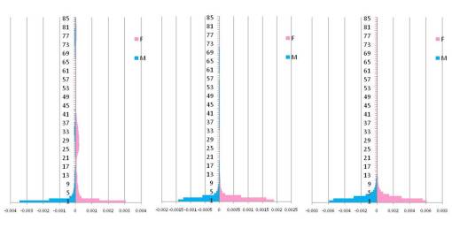
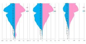
For example, the following is a theoretical population with N = 10,000,000.  The first series of graphs depict a population with original N, theoretical N, and reduced N.   This production of three different populations is presented for several reasons.  The original N is provided for comparisons with the next two analytic versions.  Theoretical N presents a theoretical population at a predetermined size , N’.   When researching several populations, it is possible to convert all populations to a standard size N’.  The purpose of this method is to make the numbers more comparable.  The original intergender age associations (M>F, F>M, ratio M:F is unchanged, relationship between Age1, Age2 . . . )  remain intact, and are applied to the new test population.  The third graph undergoes the same modifications in N or N’, but the final N” allows for statistical analyses to be performed using an equation that applies best to smaller values.   The assumption of this latter step is that if statistical significance exists with the much smaller population, and that small population represents the much larger population (since it is derived from this original population it does), any resulting statistically significant outcomes in the small group are going to demonstrate much more significant results with the larger groups of identical distributions.

.

For any study involving large masses of people, “regression to the means” rules apply.  The larger the population, the more likely your population represents the national standards.  Given a national population of 350 million, a sampling of 17% of that population or more is likely to represent the entire population’s features.  It is very hard, if not impossible to mistakenly selection a large chunk of the outliers (millions of outliers) when tens of millions of lives are being assessed.  Regression to means standards imply that large population data reviews become very stable as N is increased, and so for statistically significant differences to be generated by engaging in a new study, a doubling of the original population size is normally required for a noticeable statistical change in numbers is to be noted.  Based on reviews of how HEDIS-like data behaves for public health statisticis, it was found that for randomly generated datasets based on people behaviors (the human error component) and IT systems programming behaviors (internal or systems error inducers), an average score of 9.735 for example for a study involving 30 M people, made change only by a tenth if that 30M is converted to 60M people tested.  Such an effort is typically not worth the time for the rerun.

This study was supported and ‘passively’ supervised (for security purposes more than methodology QA related purposes) by former Perot Systems (now Dell Perot), and internal IPA and IT monitoring groups from 2004 to 2005.  All reports generated since then follow previously agreed upon institutional and federal program IP and PHI rights and regulations.  Datasets have been slightly modified without modifying statistical outcomes.  Data sources have been renamed and/or provided with a unique thoretical identifier of data content.  Only age and gender identifiers are presented in the original format.

.

HEDIS/NCQA Studies

.

Part III.  Evaluations based only on Prevalences

Stages in Life and the Progress of Disease

There are specific stages in life during which certain diseases tend to appear and prevail.  This way of interpreting disease and age resembles the teachings already out there about psychological stages in life and how conditions can progress eitehr into some sort of behavior and psychological malady, and then progress into a physiological problem with an possible neurochemistry phenomenon underlying the conditions, and/or develop more aggressively in this physical disease direction retuling in a condition which manifests itself very physiologically and in turn behaviorally and cognitively.  The psychiatric interpretation of disease that manifest in such a way might state that a particular condition is completely genetic or organic and of neurophysiological, neurochemical cause, whereas a psychological interpretation might state that a condition is manifesting itself as a result of the sociocultural setting and mindset of the individual with that particular manifestation, syndrome, behavioral problem, psychiatric condition, or predefined ICD defined diagnosis, what have you.

In physical medicine, there is also this way of interpreting diseases based on behaviors that are linked to age and gender and the surrounding environment.  Some of these physiological manifestations occur regardless of how we behave and act, others are in part a consequence of our behaviors and misbehaviors and the way that we live, but also biological in nature and manifestations as well.  Still others are almost completely a manifestation of the fate of where and how we live, appearing as a consequence of our reactions to our environment.

We can review diseases in people in a fashion that takes this varying ranges of responsibility for illness, varying from innocent to not-so-innocent reasons for pathogenesis.  By this method, the following age ranges and disease types can be defined:

1. Newborn diseases, due almost completely to the physical state of a person and his/her exposure to the environment
2. Childhood diseases due to environmental causes, with some human-generated causes for increased risk of disease development
3. Late Childhood-Early Adult age diseases due to a combination of physiological, psychological and behavioral factors
4. Mid to late Adult age diseases introduced due to complex genetic, physiological, psychological and behavioral causes, along with age-linked causes beginning to appear in the scenario as well, in particular as unhealthy chronic disease manifestations
5. Late to Very Late Adult (Elder) age diseases due to progressive disease complications, mostly linked to chronic disease related side effects, complications and physiopathologically induced somatic and psychiatric changes.

The above ways in which disease and the aging phenomena impact the body result in particular age-gender pyramid shapes, that make the progress of a long term disease understandable and often very predictable.

The amazing thing about this way of interpreting disease and predicting health is how recurrent these characteristics or traits related to a particular ICD type between seemingly unrelated disease phenomena.  Due to the way in which we classify disease, we often define all of  the baseline features for a disease, for which reason we have a hard time seeing the link between two diseases in two completely different physiological,  organ systems.  Is it possible for diseases that occur in midage in the gastrointestinal system could have some basic human physiological, environmental and behavioral features that overlap with a completely different organ system such as somatic pain and dermal sensitivity; for example, such a correlation if it does exist would suggest that GERD and Irritable Bowel Syndrome have some cause effect relationships directly linked to fibromyalgia.

Newborns and Young Children

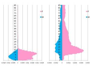
The above charts represent prevalence rates, which is to say there are the numbers of individuals afflicted, diagnosed or under surveillance for a particular condition/ICD at the “Newborns/Young Children” age range.  Without revealing the exact diseases or ICD identifications, the first condition to the left is one which occurs primarily right after birth, and decreases rapidly with time soon after birth.  Notice there is a slight rise in prevalence in the females more than the males between 20 and 30 years of age as well.  This tells us that such a condition does not only occur right after birth, but also rarely recurs in the older patient.   The fact that it is rapidly reduced in rates by the time 3 years of age is reached suggests this has something to do with environmental exposure.  It could be a condition that ensues after environmental exposure such as an infection or infectious disease state, but one which is very rare to be seen in adults.

The second condition is a typical childhood related infectious phenomenon.  Its peak is at the 1-2 year period, reducing more quickly after 9 years of age, and then plateaus at very low levels in individuals between 20 and 45 years of age.  This would be suggestive of a disease that is environmental and/or infectious based, with limited tendencies to develop a secondary peak in the younger adult years.  In the case of an evironmental diseases, this means that the body in young adults has perhaps completely adapted to the disease related problem and its causes.   For infectious diseases, this behavior would suggest that immunization either remains effective past the age of 18 and does not require some sort of revaccination, or whatever physiological, anatomical and other conditions that made the young child very susceptible no longer exist in the adult body, such as an immature immune system.  We know this is a disease related solely to the surrounding settings since it does not peak at <1 years of age like the prior.  Unlike the prior, which initiates immediately after birth, this requires some sort of human and/or environmental intervention for the condition to initiate its pathogenic process.  This minor difference in the 0-2 year old age group counts is very important to better understanding the disease or medical condition and its cause and effect relationship with the human body and with people.

The third condition is a genetically based condition which normally is diagnosed immediately after birth, and tends to have increased prevalences peaking at 8 years for males, 2 years for females.  The reason for this difference is uncertain.  Some human behavioral and environmental engagement processes are required for the condition to set in.  Notice also the secondary peak in the male population at about 20-22 years of age.  This suggests that there is a tendency either for the disease to become more likely to manifest in the early adult years, or for young adults to suddenly become more susceptible than they were during their teenage years, like when a childhood immunization wears off and requires revaccination, or this takes place due to a number of features involving lifestyle, physical body and environmental changes, and the effects these have on the genetic nature of the individual.  In cases where genetics has the effect of lessening the survivability of a body, we would expect to see this sort of reduction in numbers begin to appear due to the mortality rates these conditions result in.  Longevity for these individuals is lessened, with few surviving after 50 years of age.   Also note, there is a small peak generated on the female side of this graph–this suggests that there is some sort of natural selection process possibly going on–these women are in their reproductive years, enabling the genetic trait to continue and express itself in the younger population.  This is no doubt a very controversial type of behavior that will be seen to some extent in many genetically based diseases.   While such cases illsutrate the value of this way of looking at disease distributions across a large population, it also demonstrates the moral and ethical problems such analyses could result in.

The fourth condition is a psychological behavior pattern that manifests itself quite soon after childbirth (>1 year of age), with female prevalence twice that of male for the 1-3 year olds, followed by two more prevalence peaks for females at 13-15 and 35-47 years of age approximately (again, reproductive years).  There is a possibility that this is a biologically-based behavior change, but much of the evidence demonstrates it to be mostly of a behavioral nature.  Any childhood cases manifested as neurobiological behaviors triggered by psychosomatic and possible endocrine causes are presumably treated effectively by 15 to 20 years of age, or the problem simply is outgrown and goes away.  Also note that during the youngest and oldest childhood years, females outnumber or outbehave males in regard to prevalence status.  There is a primary peak in prevalence at ages 2-3,  another at 10-11, and a third at 37-42.   Performing a statistical test would demonstrate the second peak to demonstrate gender-defined rate differences.

Three Progressive Conditions

The next three ICDs are for genetically based syndromes or diseases, which are almost immediately diagnosed but tend to progress in life, and as a consequence even undergo a late diagnosis in some cases.  It is important to note here that there are a variety causes for pyramids to be generated in some particular form.  The attempts made here are to retain objectivity with the evaluations of these results presented, with a little subjectivity added in to disguise the true causes for the conditions illustrated.  Suffice it to say that this method had been run on hundreds of conditions enabling some ofthese differentiations to be developed, but not revealed too much right now due to IP related topics.

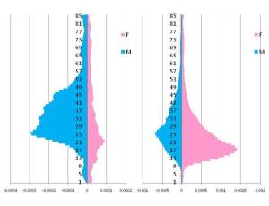
There are several features here with genetic diseases that are possibly tied to natural events, normally not evidenced by past work methodologies.  Nature has its (her) way of varying events over time as if in some sort of step-wise, undulating manner, which is that these three conditions demonstrate.   The genetic shift cocnept is well defined in past writings, in which a particular trait moves around a population rather than stay within just one narrow band of population groups that are somehow genetically defined.  It may be the disease itself and its genetic requirements, or population behavior fluctuations seen at the gender level that result in these flucatuations.

This may also be a side effect of the methodology I employed for evaluating the data that could be the cause for these undulations.  The undulations from one gender to to the next are seen with the first scenario to the left, for ages 12 to 45.  In the first graphed example, this could be due to artifical peaks displayed at 2, M, 8 (F), 12 (M), 22 (F), 27 (M), and 35 (F).  The second peak shows some smoothening of these peaks, even though they are much greater in number (this disease is rarely according to x-axis figures, but more evenly dispersed in terms of 1-year age brackets according to the figure.)  The third peak represents the smoothening out of the curve once large enough numbers of people are graphed and evaluated using the formulas that were developed.

This makes the first two peaks interesting but not necessarily something reportable with much certainty and reliability.  The third however is very reliable, and demonstrates important age peaks for the condition for separate age brackets, male versus female.  If this third peak represented a physiologically-linked genetic disorder, we see considerable gender specificity for the 21-28 year old age group–suggesting something that happens with males is creating an increased incidence.  One the other hand, sociocultural settings and the behaviors linked specifically to men may have some impact on developing this peak.  If this disease were of a psychological or mental health nature, this would be an intersting finding to report and follow up on.  Like several other diseases that exist with this same type with gender-specific age-linked prevalence outcome, there is a much larger peak for younger women than there for the mid-age large peak for men.  Women are perhaps more likely to be biologically different than men once menses begins, suggesting this is sociocultural caused age-gender relationship at least in part, and possible a directly or indirectly link genetic condition, which the medical problem is most commonly thought to be related to.  The larger peak in women in mid-childhood years could also be due to selective examination of potential victims of this condition-meaning women are more likely to undergo visit-related care and pharmacologiucal treatment than men, until the men reach 23 years of age, then they outnumber to women in the medical books.

In sum, the conditions progress from left to right as extremely rare to moderately rare.   These syndromes are mostly recognized from birth on, and tend to manifest themselves in females at one stage in life and males in two or three others.  The rarest condition on the left tends to be more fatal than the other two, but this might also be a result of its overall scarcity as well.

Mid- to Late Childhood Diseases and the Environment

The “Environment” related to health in children has two major parts to it.  There is the standard physical environment and its relationship to childhood health that we recognize, and there is the sociocultural environment that has an impact on childhood health.  These two environments are  very interaction and become increasingly interactive as the child develops a better understanding of his/her place and role in each of these and adopts new habits and behaviors in response to this learning experience.

In the next health pattern we have two medical problems, one age defined as involving a child, the other used for but not restricted to the age of an adult (>17).

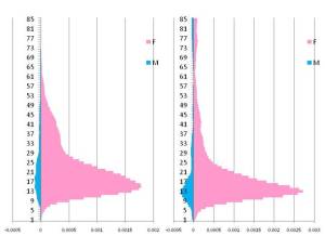
The continuation of this problem well into adulthood suggests a condition that is not age-specific and biological.  Instead, it is probably psychosocial in nature, with age acting as a determinant due to higher frequencies for specific age ranges.  Notice the significant difference in gender distributions for the second example.  Since biological is ruled out, this represents a gender related indirect lifestyle and environmental influence as being a possible cause, of an age-specific socially predictable human behavioral cause.  For both examples above, female related events significantly outnumber male-related events.

There is also a systems related effect that is responsible for the sharply define cut off for the left condition or ICD, and the well-dispered age distribution for the second condition or ICD.  The first is defined as a child syndrome–so age is a limiting factor in how it is counted in the population pyramid program.  The second demonstrate a tendency for people to not always use the terms “child” or “childhood” as a part of their diagnostics logic.  The “second adult” condition continues well into the later years of life.  Also note that there is a very gender-specific differences from teen age years on, and then a slight leveling off of the incidence rates across genders, with females slight greater than males.  Again, this is a behavioral psychology condition being evaluated for the two age ranges and is used in order to demonstrate how the judgment made of risk (by the PCP and data tech) can impact results.  These two ICDs are normally not evaluated as a single condition due to underlying sociocultural meanings attached to each.  Each has a distinctly different preventive methodologies that have to be engaged in when their rates are increased.  So the two are typically not evaluated together, and the young cases of ICD#2 are typically not included in the ICD#1 pool, although this could in theory be done for such research.

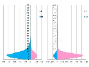
These next examples (charts above) detail a behavioral-cultural syndrome and a biological-preventible infectious disease condition.  Both have gender-specific targeting taking place.  That with the socially defined behavioral-cultural causality is gender targeted due to social reasons, which require a unique form of intervention process.  The infectious disease gender-differences for the other conditions may be culturally based or human behavior and attitude/culturally based.  In other words, certain aspects of the gender defined lifestyle relate back to likelihood of infection and spread versus the other which shows a likelihood of having culturally defined gender specific actions impacting the distribution pattern.  There is no difference in age-gender relations for a non-sociocultural event, for its causes are completely environmental and naturally based.  Unless the environment and nature are impacted by gender, age distributions are identical for conditions without the prejudice of age playing a role in the condition.  (The one of the left is sociocultural, that on the right is due solely to natural features and human physical state.)

The intervention processes for assisting in each of the two above scenarios have obvious differences.  The second ICD requries considerable efforts be made at the psychological-counseling level.  The first problem or condition requires more some physical form of intervention focused on disease prevention and physical treatment, but may have a sociocultural-behavioral component to it as well  This sociological interpretation is suggested strongly by the great reduction in this condition that aoccurs by the early 20s.  Medical conditions that prevail during the early years of life tend to be related to exposure to environmental features, for which biological and behavioral prevention practices have not yet been fully developed, or the condition has a reduction in prevalence due to early years fatality, which is not the case for this condition at all.

Late Childhood/Early Adult, or Young to Middle Adulthood

The teenage-young adult years are usually the healthiest years.  The more common ailments during these years are going to be socioculturally caused or predicted, physical ailments linked to social activities and the body’s state, and at times early or continued onset of a chronic disease that impacts these years of life.   Those diseases specific to these years, demonstrating a tendency to go away, are infrequent in the ICDs.  These are also not included much in the standard HEDIS and NCQA study options reviewed elsewhere during the course of this work, and are only on occasion included in regional and state-requested or overseer-recommended studies of Medicaid and Medicare patients.

The following are two very strongly gender-linked STDs, meaning that they show a tendency to favor one sex or the other in the clinical setting.  We know from other STD studies that some gender-related diseases and gender-favoring STDs are tested for specifically in just one population or the other.   These diseases are cross-gendered and treated and tested for in both genders, but with tendencies to demonstrate tendencies to present clinically for one more than the other.

The following pair of conditions common to and strongly linked to late teenage-early adult years are as follows.  They are very closely linked to each other, are strongly gender linked and behavioral in nature, with one demonstrating a more aggressive behavior with tendencies to appear into the later post-early adult years.  These are examples of two purely sociocultural conditions induced by personal behavior changes, with minimal linkage attributed to genetic cause (although this will no doubt change due to changing, increasing biomolecular technologies).

The numbers of male cases for both of these conditions also suggest that it is unlikely a genetic cause exists.  The possibility of genetics causes is not totally eliminated from the possibilities, but based on the previously described examples of genetic onset diseases, we expect genetic diseases to become progressive once they develop (some do develop or get diagnosed only at later ages), and either cause a mortality that results in reduced prevalences for older patients, or continues to show increasing prevalence as the older age groups are evaluated.  The narrow age band for prevalence in males for these two ICDs suggests a culturally-induced change occurs–these people no longer have that medical problem once they reach their late 20s and are required to be ‘more productive members of society’ (using the common paradigm and lingo).  The first condition, the worst of the two, has a malingering age-related incidence curve; the second has a very naroow band, again link to sociocultural definitions, interpretations and related human behaviors.

.

Middle to Late Adulthood

The middle to late adulthood years should be interpreted behaviorally and socially as the peak periods of cognitive behavior, physical and mental work productivity, high rates of healthy or recreational as well as unhealthy behaviors, and high stress related disease like consequences due to the lifestyle decisions that have been made are actively and regularly engaged in.

The diseases that present themselves during this age band can be interpreted as socially defined events, often even outweighing the biological nature of their onset.  This could be interpreted as the psychosomatic period of life, with peaks for those ages and disease patterns most often linked to psychosomaticism (as defined especially in the 1940s and 1950s, and perhaps early 1960s).  The contemporary medical philosophy relates many of the contemporary diseases with established pharmacological therapies recently developed.  These unique neurochemical explantations did not exist during the 1940s to 1960s when a lot of the diseases we see with this midage peak had a link to some sort of psychosomatic origin.

For each of these conditions there is a peak age followed by a drop in prevalence (remember, relative prevalence rates use a formula that automatically corrects for this annual mortality rate).  This drop in prevalence is due to reduction in psychosomatic behaviors, perhaps as a result of age-specific sociocultural changes expected with the post-retirement years.

The following is a basic form these kinds of conditions produce when evaluated using the new statistical method.

The following are examples of the types of outcomes generated with this formula and methodology (just relative prevalences are displayed):

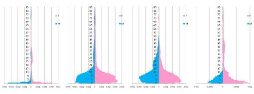
Notice how the first two demonstrate relatively early onset, one with relatively early reduction in prevalence for assorted reasons, the other due to its early mortality.  In the second example there is a significant difference in relative prevalence for deaths during the reproductive years, with males more likely to die due to this problem, ten years before the women experience the mortality of their condition.   If this was a behavioral psychology form of disease, this would have social implications in needs of further pursuit.  If this were a genetically-based disease, such a finding could have tremendous moral implications.  If it were some physical disease brought on by health related activities and behaviors, its sudden changes in mortality for men versus women at 20 years of age may be preventable.

The third example above is a disease with primary manifestations in the middle years of life.  Like the first its relative prevalence for females is greater than that for males.  The question to ask is why the reduction in prevalence from about 45 years of age and older?  Since these are prevalence rates based on gender-age-adjustments, it represents a true reduction in mortality rates from 45 years on.  This condition is a physical manifestation with possible environmental and mental health related autoimmune related causes, implying the gender differences are complex and hard to define, but result in a reduction in mortality rates in 1-year intervals from 45 on.  The slopes for male versus female prevalence rate changes pretty much remain identical and unchanged for the remaining lifespan, until the two rates are once again equal.

The following are life long conditions with age demonstrating a direct relationship to risk.  Individual survive a long period of disease, but then due to mortality changes begin to show a reduction in relative prevalence as age increases.  These are 3 of the most common causes associated with mortality and quality of life during the midlife and older years.  These curves are identical for a number of other similar chronic diseases that exist as well, with similar mortality relative prevalence rate age-gender relationships.

.

Late Adulthood to Elder

There are numerous diseases that begin to appear in increasing amounts with old age.  These include the common degenerative diseases and well as complications brought about on by some very common life long lifestyle practices and the related poor health states.

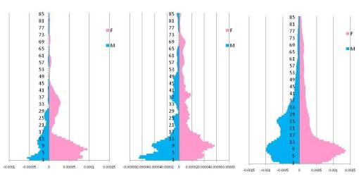
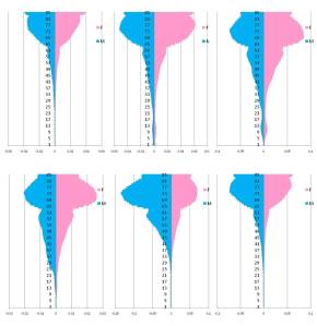
The first and last of the above medical conditions are truly progressive and are due to non-fatal illnesses that result in increased morbidity due to aging.   There is very little reduction in relative prevalence as the age continues to increase to the point of 85 years.  These are conditions that people with a disease experience as a consequence of lifestyle, made worse with aging due to lifestyle practices.  These individuals do not suffer any increase in mortality rates due to this part of their medical history, but quality of life is reduced.  Examples of these secondary disease forms that prevail with older ages (not necessarily illustrated above) include such health changes as onset of retinopathy, renal failure, end-stage renal disease, thrombocytopenia brought on by long-term prescription drug use, disseminated intravascular coagulation, peripheral neuropathy, hepatic sclerosis, portal vein shutdown, intravascular coagulation, etc. etc.

The remaining charts represent a decrease in prevalence as age increases.  This suggests the greatest morality takes hold at the max values for both sides of the above pyramids.  Charts 4 and 5 demonstrate slight gender-specific favoritism regarding mortality rates.

Examples of these diseases are syndromes and conditions more like to be associated with older age groups, like hypertension, diabetes and heart-disease induced medical conditions ranging from retinopathies, to organ failure, to onset of severe cardiac problems and disturbances.

More on Gender Specificity

Some diseases are logically gender specific.  Breast cancer is primarily female in nature (although of course male cases do exist!), and specific anatomically related conditions or health related activities are gender specific, like child deliver or a type of infection known as balantidiasis which only involves the penis.

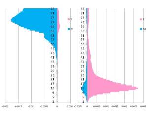
The gender-specific condition on the left is an occupational disease that relates almost entirely to men.  The condition on the right is a sociocultural behavioral disease or syndrome related mostly to women.

These two conditions have very different temporal features.

The first is of old age occurence, and notice it continues past retirement years, and has a reduction in survival rates after the age of 75.  This condition is brought on occupationally by long term occupation related risks, resulting in physical deterioration in the later years.  Examples of this type of problem could include such medical problems relate to long-term radiation exposure in a male dominant job, long-term exposure to a primarily males only carcinogen, or long-term male-specific environmentally induced disease problems, such as physically compromising, high weight related occupational risks.  There is a 20:1 ratio for frequencies of men:women.

The second condition occurs in women and had an age distribution much greater than that of men.  Interestingly, the peak year is 15 or 16, with this large peak reducing in size quickly by the time the early 20s are reached.  There is a 6:1 ratio of women:men.

Other Statistical Numbers-derived Behaviors

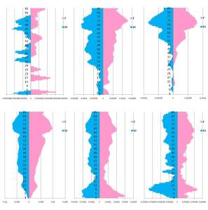
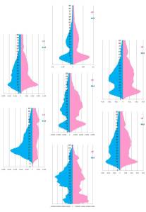
These structures have a tendency to demonstrate gender crossovers, resulting  in age groups in which only one gender is affected by a condition.  When total numbers of cases are small, this might be explains as a result of small n and large variance.  But these undulations are seen as well for larger n’s as well, suggesting there is another cause for this phenomenon.  The third example below of a very popular condition nearly extinguished over time demonstrates one of the best examples of an undulating pattern.  The alternating male-female pattern change suggests a possibility for gender specific genome-related changes for the organism responsible for the condition, i.e. preference for one gender over the other, cycling back and forth during the final years of existence.

.

Examples of Application

STDs.  Your company decides it wants to produce a more effective program for reducing sexually transmitted disease (STD) rates.  The current prevention program in place mails letters to people when they reach 18 years of age and continues to monitor and periodically mail out reminder letters to people who are not married and are between 20 and 45 years of age.  For this age range this means that 1.5 million letters are sent per year at reduced costs for bulk mailing, but still costing about $250,000 per year for the mailing, and another $500,000 in printing and administrative costs, costing you approximately 50 cents per letter.

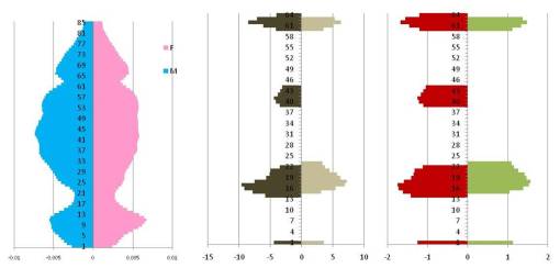
When you review the population health features  for this particular STD you find that the following age-gender distribution in prevalence exists for this particular STD.

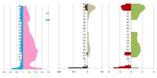
The above tables illustrate that women experience this condition much more than men, approximately 10 times as often relative to men at the age of 25 years of age, the peak year for people with this diagnosis on record.  Age ranges that are statistically significant are illustate on the middle figure, and show that there is little to no statistically significant prevalence rates in men other than at the age of 14 to 16 years of age.  For women, there is a large age range where the rates stand out as being statistically significant, with the third graph emphasizing the scope to which the interventions to be developed need to be implemented.

The following are the results inferred by this method of modeling the age-gender relative prevalence rate statistics:

An intervention that targets teens has to be developed due to the bi-gender statistical significance illustrated for individuals 14 to 16 years of age.  Due to early onset of this problem in the female cases, you decide that this program perhaps should also have some activities in place as early as 12 years of age as well.

In addition, the highest risk group is the female population ranging in age from 17 to 36 years of age, with a possible risk group also found in the  48+ year olds for females, 59+ year olds for men.   These specific groups of people are targeted, with very different methods taken to interventions targeting men and women, and young to middle aged versus old.   Notice there was no need suggested by these statistics for targeting nearly all middle aged men and all women between the ages of 37 and 48.

This redirects the cost of your intervention program, allowing it to more effectively target age-specific group types.    Chances are your method of engaging in these activities will adapt the traditional mailing method, but more selectively choose the types of members you mail to, cutting the cost for this mailing in half.  This money can then be redirected at targeting older people married or unmarried, either through bulk advertising means or by way of selecting the highest risk individual based on marital status.

Psychologic and Psychiatric Disorders

.

Conclusion

This methodology was created for accurately analyzing and predicting population health for programs designed to developed more precisely targeted intervention practices.  With the data on exceptionally large populations now available  to research in public health, the method developed for population health research enables new measurement techniques to be implemented and employed for the development of more cost-effective intervention programs.  The methodology presented above is based upon the mathematics developed for evaluating population curves, using a very detail-oriented formula approach previously employed for such studies involving transect analyses and facial identification software techniques.  The results of this work were developed into teaching tools, which were never presented in the academic setting.   The mathematical details on the above methodology have since been restricted in distribution due to IP ownership concerns and issues.

The above applications of this methodology serve to illustrate the various ways this methodology can be applied.  In essence, this methodology allows for reviews of unlimited amounts of data linked to age-gender as independent variables.  This methodology in the above examples was applied to two fields with large numbers of participants–sports and recreation, and population health.  These methods could also be applied for patient studies involving any large-scale data gathering system related to topics as unique as food marketing and consumer history, gas or petroleum fuel utilization as an areal-cost related feature, or assessments of detailed regional changes made over time related to local demography, income-family histories and political party classifications.  This methodology is basic and therefore has numerous applications for use as a highly realistic and useful applied population research methodology and tool.

ADDENDA

EXERCISES

The following series of questions were developed back in 2004/5 for the educational program I wrote up on my results, used to teach students and some data entry specialists how to read and interpret the above types of population pyramid graphs. [Tentative class schedule will be posted separately once I find it.]  For much of the training see all pages related to https://brianaltonenmph.com/biostatistics/quality-assurance/population-disease-monitoring-the-elephant-of-public-health/)

MIDTERM

1.  What are the makings of a population pyramid?  What are the format standards (include standard color coding of text/numbers and horizontal bars, inclusion of legends, etc.)

2.  What are the differences, the pros and cons, regarding how we demonstrate age-gender relationships?  Define this for 1, 2, 5 and 10 age range horizontal bar increments.  Which are used most commonly and when?

3.  What are the main advantages and disadvantages to small group analyses?  What are the population and group min-max limits pertaining to this graphing technique?

4.  Define a standardized uniform group analysis technique.  How is this technique modified for the special format problems that varying populations present analysts with?

5.  What N defines the limit as to whether or not 1-year age bands can be used?  What min and max define the formula multiplier employed for this type of uniform group analysis technique?

6.  What is the name of the technique employed for this analysis.  What standard formula does it make use of?  Define how it is employed.

7.  Provide one or two research questions this methodology might be applied to.

8.  Define your dependent and independent variables for this research.

9.  Define how to employ this math modeling technique to two dependent variables, treating one as a dependent variable.

10.  How would you use the above methods to correlate cost to age-gender variables.

FINAL

1.  Define and name the stages each of  the following charts best relate to.

2.  Do the following represent maladies that require preventive or palliative treatment forms to be established?

3.  Define the age groups in the following disease types for which prevention programs can be developed.  How would you apply the standard disease prevention practices differently to each of these age groups?

[insert Disease A, B, C, D]

4.  For the above four graphs, which of the four most likely represents a genetic disease with a relatively high mortality rate?

5.  Which represents a disease that is life long and relatively speaking is the least fatal of the above four illustrated?

6. Which represents a disease that is more than likely unpreventible in terms of onset and treatment, and generally speaking is not very fatal to its primary age group?

7.  Is the follow graph most likely indicative of a biological-physiological malady, a mostly behavior-psychological malady, or a mixed sociocultural, physical and psychological malady?  Based on this graph, how might you describe your treatment for this disease were it your responsibility to treat it as a only as biological and physiological event?  as a purely psychiatric event?

8. Which of the following best represents an event that presents itself mostly as a young to midlife event?  What is the most likely type of disease or disease related behavior related to this malady or condition?

 

“. . . the solutions to our problems lie outside the box.”

Aviation Week & Space Technology, July 1975